- Panyu District, Guangzhou, Guangdong, China
- 2044, 2nd Floor, Yayun Avenue, Dalong Street
- whatsapp:
- +86 13265357928
SPC Blog
Should Manufacturing Companies Still Implement SPC Amid Economic Downturn and Poor Business Performance?
In situations like economic downturn, poor business performance, insufficient orders, and idle production lines, besides personnel optimization and cost control, let's examine what SPC can bring to enterprises from a quality perspective.
I. Improved Performance
SPC provides objective, quantifiable process capability data, demonstrating the stability and high standards of production quality.
It enhances customer confidence, especially for customers with high quality requirements (such as those in the automotive, auto parts, and electronic chip industries).
SPC is the "key" to entering high-end supply chains. Without implementing SPC, companies may not even be eligible to bid. Furthermore, customers tend to choose suppliers with stable processes because it saves them on inspection and management costs.
It reduces customer audit risks. A mature SPC implementation system leaves a professional and reliable impression on auditors. Successfully passing audits reduces the risk of customers demanding corrective action or even canceling orders.
Compared to companies that don't implement SPC, they are more likely to obtain better audit scores and higher order quotas. It also fosters long-term partnerships, making customers less inclined to switch suppliers easily.
II. Cost Control
1. Reduce Scrap and Rework
Implementing SPC allows for real-time monitoring via control charts, with immediate alerts for any anomalies, minimizing the generation of batches of non-conforming products. This directly reduces raw material waste, labor waste, and the cost of handling scrap, while improving the first-pass yield.
2. Optimize Process Parameters
By analyzing control charts and process capability indices, key variables affecting quality can be identified, thereby determining optimal production conditions. This reduces quality problems caused by parameter fluctuations, resulting in more stable and efficient production.
3. Reduce Inspection Costs
When the process is under statistical control, the need for full inspection of the final product can be reduced, replaced by more economical sampling inspection. This saves significant investment in manpower and inspection equipment.
III. Improve Human Resource Utilization
1. Fully Utilize Idle Manpower
When orders decrease, the "waiting time" for operators, technicians, or quality personnel increases. Sometimes, large-scale workforce optimization isn't feasible. Implementing SPC allows idle staff to learn SPC theory and participate in quality analysis and improvement processes, avoiding wasted human resources. This ensures employees can still create value for the company even with insufficient working hours, preparing for future order peaks.
2. Enhancing Employee Skills
SPC requires employees to learn statistical thinking, data collection, and problem-solving. Cultivating a core group of talent with data analysis and continuous improvement skills is an invaluable competitive advantage after economic recovery.
IV. Laying the Foundation for Long-Term Development
SPC provides objective data for problem analysis, rather than relying on experience or guesswork. This ensures management's improvement decisions are based on facts and data.
SPC can drive a shift in thinking from "producing products" to "producing qualified and stable products," cultivating a quality-conscious mindset across all employees. It improves the overall management level of the enterprise, laying the foundation for future automation and digital transformation.
Building competitive barriers, especially during economic downturns when competitors may choose to reduce quality management investment. Implementing SPC at this time often results in higher cost-effectiveness and more stable quality, seizing market share. This creates a unique competitive advantage, preparing for rapid growth after economic recovery.
What should we do if the customer requires the immediate implementation of SPC process control during a factory audit?
Many factories face customer audits that require them to implement SPC (Service Process Control) as soon as possible, which presents a significant challenge. Implementing SPC doesn't seem like an easy or quick process. So what can be done?
Using Excel is incredibly time-consuming and doesn't allow for comprehensive SPC process control.
Is there a way to achieve comprehensive SPC process control that is both cheap and fast?
This requires that:
· SPC software can acquire test data and operational data through multiple methods;
· It should be ready to use immediately upon deployment and installation;
· It shouldn't be used by just one person; it should be usable by both the quality department and the production department;
· And it shouldn't be too expensive, costing hundreds of thousands.
In addition, essential SPC functions must be included, such as:
· Support for various SPC control charts
· Support for eight major anomaly detection rules and custom rules
· Support for process capability statistics such as CPK, PPK, CPM, and CA
· Real-time viewing of SPC analysis reports
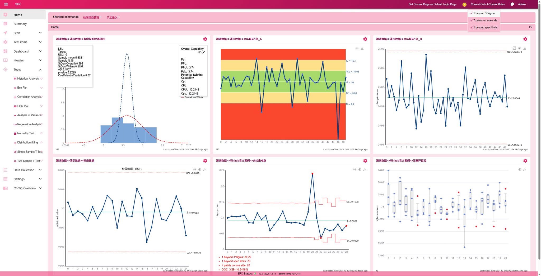
· SPC dashboard functionality
· Ideally, backend monitoring with notifications via email, WeChat Work, etc.
It seems that to meet all the above requirements, it would require at least hundreds of thousands US dollars plus one or two months of on-site implementation, which is quite difficult in terms of both cost and time.
Therefore, we recommend our Simple SPC, which has the following features.
· Deployable in just one day.
· Price in the tens of thousands US dollars.
· Unlimited users, unlimited online users, unlimited monitoring points, unlimited dashboards; one account per user.
· All users access the service through a browser.
· Server license, one-time lifetime license, no annual license fee.
· Supports SPC control charts: I-MR, Xbar-S, Xbar-R, MR-R/S, NP, C, P, U.
· Fully supports the eight standard SPC anomaly detection rules (and custom anomaly detection rules).
· Multiple data entry methods: online manual entry, online Excel import, HTTP interface synchronization, TCP server mode, MQTT mode, OPC data acquisition.
· One-click output of comprehensive SPC analysis reports: control charts, normality tests, rainbow charts, box plots, distribution fitting, process capability analysis histograms, machine learning outlier charts, capability comparison charts, data summaries, large model interpretation.
· Create any number of SPC monitoring dashboards: dynamic dashboards, comprehensive dashboards, statistical dashboards, which can include SPC control charts, rainbow charts, histograms, and box plots for any testing item, ideal for workshop dashboards.
· Backend monitoring: SPC control chart outlier detection, CPK and PPK anomaly monitoring.
· Notification channels: email, WeChat Work, DingTalk, Lark, MQTT, API.
· Real-time automatic updates of control charts.
· 11 language versions.
· Multiple analysis tools: CPK tool, regression analysis, correlation analysis, normality tests, one-sample t-tests, two-sample t-tests, distribution fitting, etc.
· Open SPC outlier detection API and other data synchronization, testing item creation, etc. APIs.
· Integrated with MSA.
· Private deployment on the enterprise intranet, data security and controllability, browser-based, no client installation required.
This is why our Simple SPC software is the first choice for our customers.
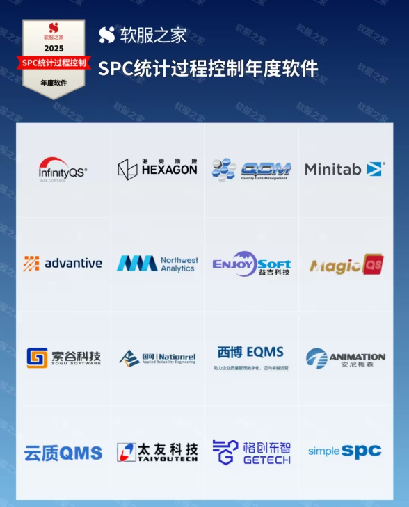
Simple SPC has been recognized for the third time as the "2025 SPC Statistical Process Control Software of the Year" by China SoftWare Home.
Since its launch in 2022, Smiple SPC has been awarded the "Statistical Process Control Software of the Year" by SoftWare Home three times, for the years 2022, 2024, and 2025. Over the past four years, an increasing number of customers have chosen our solution.
· SoftWare Home | 2025 SPC Software of the Year List (Rankings are in no particular order).
Giving SPC AI Wings: DeepSeek Enhancing Efficiency and Depth of Quality Management
When we talk about Artificial Intelligence, do star Large Language Models (LLMs) like DeepSeek pop into our minds? They can not only engage in intelligent chat and write articles automatically, but even help us program efficiently. And when it comes to industrial production, we often focus on quality management tools like control charts and process capability analysis. General-purpose AI models (represented by large models such as DeepSeek, ChatGPT, and Gemini) represent the most cutting-edge intelligent technology of the information age, while Statistical Process Control (SPC) embodies the spirit of continuous improvement in product quality from the industrial age. Many people wonder how LLMs will replace SPC. Today, let’s discuss what general-purpose AI models (especially large models like DeepSeek) and SPC are all about. More importantly, let's explore whether we can leverage the “superpowers” of LLMs like DeepSeek to give traditional SPC analysis a major upgrade and usher in a new era of intelligent quality management!
First, we need to clarify the essence and respective focus of general-purpose AI models and SPC. Although both are important tools and methodologies, they have significant differences in application areas and core functions. Understanding their essential differences and possible connections will be very helpful for us to better utilize them in practical work.
General-purpose AI Models (Represented by DeepSeek, etc.): Powerful pre-trained language models, with natural language processing (NLP) at their core and particularly outstanding code generation capabilities.
General-purpose AI models might be more familiarly known by their “stage name” “GPT (Generative Pre-trained Transformer)”. Now, more representative examples might include a series of emerging powerful models like DeepSeek. These models are all “leaders” among pre-trained language models. General-purpose AI models are powerful pre-trained language models. Their core advantage lies in their expertise in understanding and generating natural language text – simply put, they are exceptionally good at “talking”. This makes them incredibly capable when handling various NLP tasks, demonstrating outstanding abilities in areas such as:
- Intelligent Question Answering: Able to understand questions posed by users and provide accurate and relevant answers, like having a "know-it-all" by your side.
- Writing Assistant: Can help users write articles, whether it's creating stories, drafting emails, or generating news reports, they can lend a hand and boost efficiency significantly.
- Code Generator (Especially DeepSeek, etc., with outstanding code generation capabilities): You heard it right, they can also write code! Especially large models like DeepSeek, which excel in code generation, and can even assist programmers in completing programming tasks, becoming a valuable assistant for programmers.
- Information Summarizer: When facing a large amount of textual information, they can quickly "scan" through it, extract key points, and generate concise summaries, saving time and effort.
SPC: The cornerstone of quality management, SPC is a quality management technique that utilizes statistical principles and methods to monitor and control production process variation, and it also needs to undergo "intelligent upgrades" by embracing large models like DeepSeek.
SPC, or Statistical Process Control, remains the “cornerstone” of quality management. It is a quality management technique that utilizes statistical principles and methods to monitor and control production process variation in order to ensure stable product quality and continuous improvement. Its core objective remains to “keep a close eye” on production process variation, ensuring our product quality is consistently reliable and can be continuously improved. The core methods of SPC include control charts, process capability analysis, and various statistical analysis tools. SPC's "combination punch" mainly consists of the following techniques:
- Control Charts: Like a "monitoring radar", they use graphical methods to visually display the fluctuations in production process data. Once an "abnormal signal" is detected, they immediately "alarm", reminding us to take timely measures.
- Process Capability Analysis: Like giving a "health check" to the production process, assessing its "physical fitness" to see if it can meet quality standards and identify areas for "improvement".
- Statistical Analysis Tools: Various statistical analysis methods, such as hypothesis testing, regression analysis, etc., are like "magnifying glasses" and "microscopes", helping us to deeply analyze process data and find the "hidden culprits" affecting quality.
The key to SPC lies in the collection, analysis, and interpretation of production process data, and taking corresponding control and improvement measures based on the analysis results. The key to SPC also lies in continuously collecting production process data, then conducting systematic analysis and professional interpretation, and taking corresponding control and improvement measures based on the analysis results. Simply put, it's about using data to speak and using statistical methods to guide quality improvement. However, in today's era of data explosion and increasingly complex production environments, traditional SPC analysis methods also face some "minor challenges":
- Slow Data Analysis: Traditional SPC analysis mainly relies on manual chart viewing and analysis, which is relatively inefficient and feels “overwhelmed” when facing massive real-time data.
- Over-reliance on "Veteran Experts": How to interpret SPC analysis results and determine improvement measures largely depends on the experience and expertise of quality engineers, and talent in this area is relatively “scarce”.
- Underutilization of Unstructured Data: Production processes generate a lot of unstructured data such as text records, images, and sounds, etc. Traditional SPC methods are not good at "dealing with" this information, which is somewhat wasteful.
Large Models (especially DeepSeek etc.) + SPC = "New Playbook" for Intelligent Quality Management? DeepSeek and other large models may become the key to intelligent upgrades of SPC.
Therefore, it's not about simply throwing a set of detection data at a large model and expecting it to automatically generate control charts and calculate process capability. Instead, it's about applying SPC tools, feeding the results data, such as control charts (out-of-control points) and process capability indices, into large models, and letting the models help us write SPC analysis reports, analyze root causes, and provide recommendations.
Large models like DeepSeek can become a “super plug-in” for SPC, enhancing the efficiency, depth, and intelligence level of SPC analysis in various aspects. How do large models like DeepSeek "buff up" SPC analysis?
Root Cause Analysis and Problem Diagnosis:
- Turning Unstructured Data into Valuable Assets: Large models like DeepSeek can "understand" and "see" various unstructured data generated in production processes, such as operator's text records, equipment maintenance logs, defect images, and even voice data. By analyzing these "edge-case" information, large models like DeepSeek can unearth deep-seated root causes of problems that traditional SPC methods "overlook".
- "Knowledge Graph" + "Expert Embodyment" + Intelligent Reasoning: Large models like DeepSeek can build a "knowledge graph" in the SPC domain, "loading" in knowledge of SPC principles, process knowledge, equipment information, historical cases, and so on. With this "knowledge base", large models like DeepSeek can perform intelligent reasoning and diagnosis, helping quality engineers quickly locate problems and even provide possible solutions as "suggestions".
Predictive Quality Management and Preventive Measures:
- "Early Warning" of Quality Trends: Large models like DeepSeek can analyze historical SPC data, learn the "temperament" and "patterns" of quality fluctuations, predict future quality trends, and provide "early warnings" of potential quality problems, giving companies ample time to "prepare for a rainy day".
- "Intelligent Optimization" Suggestions for Process Parameters: Based on a thorough "understanding" of SPC data and process knowledge, large models like DeepSeek can intelligently recommend optimal process parameter settings, making production processes more stable and product quality even better. This is much more powerful than the traditional SPC's "hindsight bias"; it directly "prevents problems before they happen"!
A More "Human-friendly" Human-Machine Collaborative SPC Analysis Platform:
- "Voice-activated" Natural Language Interaction Interface: Large models like DeepSeek can create a natural language interaction SPC analysis platform. Users can directly use "plain language" to issue commands to complete data queries, chart generation, anomaly analysis, and other operations, greatly lowering the threshold for using SPC tools and allowing more production personnel to participate in quality management.
- "Intelligent Assistant" + "Expert Empowerment": Large models like DeepSeek can become "intelligent assistants" for quality engineers, assisting experts in complex SPC analysis work, providing "one-stop service" such as data interpretation, report generation, and solution suggestions, improving expert work efficiency and decision-making levels, and also better "passing down" the expert’s knowledge and experience.
Looking ahead, the "marriage" of large models and SPC is definitely a major trend in intelligent quality management. The key to SPC lies in the collection, analysis, and interpretation of production process data, and taking corresponding control and improvement measures based on the analysis results. As large model technology becomes increasingly mature and widespread, we have reason to believe that large models will play an increasingly important role in SPC analysis, driving quality management from traditional models towards an intelligent, preventive, and efficient “fast lane”, ultimately helping companies achieve higher levels of quality excellence.
AI-Enhanced Statistical Process Control (AI-SPC): Revolutionizing Quality Management in the Era of Smart Manufacturing
In the age of smart manufacturing, AI technology is profoundly transforming the field of quality management. This article introduces an artificial intelligence-based SPC analysis method (AI-SPC), which utilizes machine learning algorithms to predict future trends in detection data, achieving more accurate anomaly warnings. This helps enterprises improve product quality, reduce production costs, and advance towards a new stage of intelligent quality management.
This article is divided into four main sections:
- Process Design
- Core Concepts
- Features and Advantages
- Application Value
I. Process Design
Below is a flowchart of SPC integrated with AI prediction:
① Timed Detection of Detection Items Requiring Predictive Model Reconstruction:
To ensure the effectiveness and accuracy of the predictive model, it is necessary to set a model reconstruction cycle for detection items. The reconstruction cycle can be set based on time intervals (e.g., weekly, monthly) or data update volumes. Model reconstruction is triggered only when the new detection data volume of a detection item reaches a preset threshold or when the time since the last model reconstruction exceeds the set cycle.
② Model Reconstruction: Multi-Algorithm Model Training and Optimization:
For each detection item requiring predictive model reconstruction, the system automatically trains multiple machine learning algorithms and neural network models, such as time series models (ARIMA, Prophet), recurrent neural networks (RNN), long short-term memory networks (LSTM), gradient boosting decision trees (GBDT), random forests, and more than a dozen other prediction algorithms and their variants. The system evaluates the performance of the trained models through cross-validation, model evaluation metrics (e.g., root mean square error RMSE, mean absolute error MAE), and other methods, ultimately selecting the algorithm model with the best predictive performance as the optimal predictive model.
③ Record and Store Optimal Predictive Model:
The system records and stores the optimal predictive model information for each detection item, including key information such as the optimal algorithm name and version, model parameters, predictive performance evaluation metrics (e.g., RMSE, MAE), and feature variables used during model training. This information is stored in the database and associated with the corresponding detection items, facilitating subsequent model calls, performance tracking, and management, and providing a basis for subsequent model optimization and performance monitoring.
④ Predict Future N Points:
Predict future N detection points based on the optimal model: According to the user-set prediction step size N (e.g., predict the next 3, 5, 10 detection points), the system calls the stored optimal predictive model to predict the data of the next N detection points and record the prediction results. The setting of the prediction step size N can be determined according to actual production needs and warning lead time. The prediction results are stored in the form of data tables or charts for subsequent analysis and display, providing a data basis for drawing predictive SPC control charts.
⑤ Merge Predicted Values with Actual Values:
Merge predicted values with actual values to construct AI-SPC control charts: The system integrates the predicted values of the next N detection points with the existing actual detection data. On the basis of traditional SPC control charts, a predicted value curve is added to form an AI-SPC predictive control chart. For example, predicted values can be added to the X-bar control chart in the form of dashed lines or lines of different colors, so that the control chart not only displays historical data but also includes predictive information on future trends, helping users to more comprehensively grasp the process state.
⑥ Execute Eight Extended Rules for Determining Abnormalities:
Execute extended SPC eight rules for determining abnormalities (including predicted values): On the basis of the traditional SPC eight rules for determining abnormalities, for AI-SPC control charts that include predicted values, the system executes the set SPC rules for determining abnormalities, such as points exceeding control limits, consecutive points showing an upward or downward trend, consecutive points on one side of the centerline, and periodic fluctuations. The SPC eight rules for determining abnormalities are a set of statistical rules used to determine whether abnormal fluctuations or special causes occur in the production process. These rules for determining abnormalities can be flexibly configured according to the quality control requirements of the actual production process to meet the needs of different scenarios.
⑦ Anomaly Warning:
Anomaly warning and multi-channel notification: When the system detects an abnormality signal in the AI-SPC control chart (i.e., the set rules for determining abnormalities are triggered), it indicates that quality abnormalities or process fluctuations may occur in the predicted future. The system immediately activates the anomaly warning mechanism and sends real-time warning notifications to relevant personnel (e.g., quality management personnel, production line leaders) through preset interfaces (e.g., API interfaces), email, enterprise WeChat, SMS, and other channels. The notification content can include: the detection item where the anomaly occurred, the type of rules for determining abnormalities, the predicted anomaly trend, and recommended disposal measures.
⑧ New Detection Data Entered:
Data-driven continuous optimization: New data updates and model self-iteration: As new detection data is continuously generated, the system continuously monitors the new data volume of detection items. When the new data volume reaches a preset threshold, the system automatically triggers the model reconstruction process (return to step ①), uses the latest detection data to retrain the model, and performs model optimization, realizing self-iteration and continuous optimization of the predictive model, ensuring that the model can always capture the latest data features and provide the most accurate predictions. The entire process forms a data-driven closed-loop system that continuously learns and adapts to new data patterns, thereby achieving more intelligent and accurate SPC analysis and providing continuous value for quality management.
II. Core Concepts
Model Management and Reconstruction: The AI-SPC process demonstrates a comprehensive design concept in the model management and reconstruction stage. Its model reconstruction trigger mechanism takes into account both time cycles and data volume thresholds, ensuring that the model can be updated in a timely manner and avoid unnecessary reconstruction, reflecting efficiency and flexibility. The introduction of multi-algorithm model training covers multiple algorithms such as time series models and deep learning models, and model evaluation and optimization are performed through cross-validation and other methods, ensuring the scientific nature of model selection and prediction accuracy.
Prediction and Analysis: The core value of the AI-SPC process lies in its powerful prediction and analysis capabilities. Multi-step prediction based on the optimal model realizes effective prediction of future quality trends, transforming quality management from passive response to active prevention. The intelligent integration of predicted values and actual values constructs AI-SPC predictive control charts, which incorporate future trend information on the basis of traditional SPC, providing users with a more comprehensive view of the process state. The extended SPC eight rules for determining abnormalities fully utilize predictive information to achieve more intelligent and sensitive anomaly determination.
Warning and Optimization: The AI-SPC process reflects the foresight of intelligent quality management in terms of warning and optimization. The multi-channel warning mechanism ensures real-time access to anomaly information, giving enterprises valuable response time. More importantly, the data-driven model self-iteration update mechanism gives the system the ability to continuously learn and evolve, ensuring that the AI-SPC system can maintain optimal performance for a long time and continuously adapt to changes in the production process.
III. Features and Advantages
The AI-SPC system integrates the advantages of artificial intelligence and statistical process control, showing the following significant features and advantages:
- Intelligent Prediction Capability: Predict quality trends in advance. AI-SPC breaks through the limitations of traditional SPC and has the ability to predict future quality trends, helping enterprises to calmly respond to potential quality risks.
- Adaptive Optimization: Continuous learning and model updates. The system can continuously learn and optimize with the accumulation of new data, and the model performance continues to improve, ensuring the long-term effectiveness and intelligence level of the AI-SPC system.
- Multi-Algorithm Fusion: Improve prediction accuracy. The multi-algorithm fusion strategy fully explores the potential of data, selects the optimal predictive model, and significantly improves the accuracy and reliability of prediction.
- High Degree of Automation: Reduce manual intervention. The AI-SPC process has a high degree of automation, greatly reducing the need for manual intervention, improving the efficiency and consistency of SPC analysis, and reducing labor costs.
- Real-Time Warning: Provide longer problem response time. The real-time warning mechanism based on prediction results provides enterprises with longer response time, helping to take measures before problems occur and reduce quality losses.
IV. Application Value
The application of AI-SPC technology will bring significant value improvement to enterprises:
- Quality Improvement: Discover problems in advance through predictive analysis. The predictive capability of AI-SPC helps enterprises move the focus of quality management forward, discover potential quality problems in advance, prevent problems before they occur, and ultimately achieve continuous improvement of product quality.
- Cost Reduction: Reduce the generation of defective products. Through more timely anomaly warnings and faster problem response, AI-SPC helps reduce the generation of defective products, reduce quality costs such as rework and scrap, and improve enterprise profitability.
- Efficiency Improvement: Automated analysis replaces manual operations. The automation feature of AI-SPC frees quality management personnel from repetitive labor, allowing them to focus more on high-value work such as quality improvement and optimization, and improving overall quality management efficiency.
- Simple SPC 4.0 – Detailed Product Overview
- Simple SPC 4.0 Official Release
- Using data to safeguard safety: Application practices of SPC in the pharmaceutical industry
- How can risks be identified in advance in automobile manufacturing? — Sharing SPC application practices
- Innovative Practices and Applications of Web SPC Systems
- Should Manufacturing Companies Still Implement SPC Amid Economic Downturn and Poor Business Performance?
- What should we do if the customer requires the immediate implementation of SPC process control during a factory audit?
- Simple SPC has been recognized for the third time as the "2025 SPC Statistical Process Control Software of the Year" by China SoftWare Home.
- Giving SPC AI Wings: DeepSeek Enhancing Efficiency and Depth of Quality Management
- AI-Enhanced Statistical Process Control (AI-SPC): Revolutionizing Quality Management in the Era of Smart Manufacturing
- General-Purpose Artificial Intelligence Models (DeepSeek, etc.) and Statistical Process Control (SPC): A New Era of Intelligent Quality Management
- Simple SPC 2.0 released, with upgraded functions and optimized performance
- CPK and PPK: Essential Questions in Quality Interviews, Do You Truly Understand Them?
- Unilateral or Bilateral: An In-Depth Exploration of Specification Limits and Control Limits in SPC Analysis and Their Impact on Metrics
- How to Calculate Control Limits for Xbar-R and Xbar-S Control Charts in SPC Analysis and When to Use Each Chart
- Is SPC or Another Method Better for Determining Batch Consistency with Standards? A Recommended Analysis Approach
- Beyond SPC Control Charts: Lesser-Known but Effective Quality Analysis Tools
- SPC is the most accessible, effective, and performance-demonstrating analytical tool in the manufacturing industry.
- How to Quickly Identify Hidden Correlations Between Test Items Using the SPC System?